BigQuery: Advanced SQL query hacks
This is a list of time-saving, cost-saving and life-saving SQL query hacks you need to know if you consider yourself an advanced BigQuery user.
Select all columns by excluding only some of them
When you need to select all the columns in the table but a couple of them you can use the EXCEPT keyword to do so:
SELECT * EXCEPT (col1, col2)
FROM `project_id.dataset_name.table_name`
Convert JSON into structured data
If you have JSON formatted text in a string column you can use JavaScript UDF to convert the JSON text into an array which will be displayed as a nested field in BigQuery:
CREATE TEMP FUNCTION unnestJson(str STRING)
RETURNS ARRAY<STRING>
LANGUAGE js AS r"""
  var obj = JSON.parse(str);
  var keys = Object.keys(obj);
  var arr = [];
  for (i = 0; i < keys.length; i++) {
    arr.push(JSON.stringify(obj[keys[i]] || ""));
  }
  return arr;
""";

SELECT col1, unnestJson(col2) FROM `project_id.dataset_name.table_name`
Define queries and static values once if you have multiple references
If you need to reference a certain subquery multiple times in your main query or have to reference a certain value (e.g. a specific date) multiple times within the main query, you can use WITH to define it as a common table expression (CTE) and/or DEFINE to define a value as a static SQL variable.
In your actual query you can reuse all these definitions just by referencing them.
DECLARE start_date DATE DEFAULT DATE('2020-09-29');

WITH

valid_dataset AS (
  SELECT *
  FROM `project_id.dataset_name.table_name`
  WHERE col1 = TRUE
),

valid_dataset2 AS (
  SELECT *
  FROM `project_id.dataset_name.table_name`
  WHERE col2 = TRUE
)

SELECT col2
FROM valid_dataset
WHERE col3 > start_date
UNION ALL
SELECT col2
FROM valid_dataset2
WHERE col3 > start_date
UNNEST will automatically CROSS JOIN results
Be careful when using UNNEST, as it will automatically CROSS JOIN the results from the parent table and the untested table. This means that results from the parent table will disappear if there are no relevant rows in the untested table.
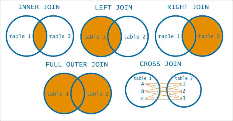
I’ve found that in most cases it would be safer to UNNEST by using LEFT JOIN instead. You can see the syntax for both options in the example below. Test this with your dataset to understand what works best for you.
-- UNNESTING BY CROSS JOIN
SELECT
  session.id as ses_id,
  h.id as hit_id
FROM
  `project_id.dataset_id.sessions` AS session ,
  UNNEST(session.hits) AS h ,
  UNNEST (h.events) as e


-- UNNESTING BY LEFT JOIN
SELECT
  session.id as ses_id,
  h.id as hit_id
FROM
  `project_id.dataset_id.sessions` AS session` AS session
  LEFT JOIN UNNEST(session.hits) AS h
  LEFT JOIN UNNEST (h.events) as e
Testing queries that will update your data (like a Pro)
When updating data with a DML SQL query (e.g. UPDATE, INSERT) you need to be very careful. The easiest approach is to use a SELECT query that matches what you want to do in your final SQL query (see example below).
-- TESTING USING A SELECT QUERY
SELECT
 additional_information,
 regexp_replace(additional_information,'Old value', 'New value') AS new_additional_information
FROM
 `project.dataset.table`
WHERE
 account_id = 123
 AND additional_information LIKE '%Old value%'

-- MAKING CHANGES WITH AN UPDATE QUERY
UPDATE
 `project.dataset.table`
SET
 additional_information = regexp_replace(additional_information,'Old value', 'New value')
WHERE
 account_id = 123
 AND additional_information LIKE '%Old value%'
But this approach is not foolproof, as there’s always a small chance to have a typo or small differences between the 2 versions.
Ideally, you want to be able to run your query, see the changes in your data, and only after you verify that everything looks OK, apply the changes! You can do that with a ROLLBACK statement!
-- TRANSACTION WITH ROLLBACK
BEGIN TRANSACTION;  INSERT INTO
    `project.dataset.table`
  VALUES ('New value', 'Another new value', 123);  SELECT
    *
  FROM
    `project.dataset.table`;ROLLBACK TRANSACTION;
Cut down query costs with Partitioned or Clustered tables
When using a DB for a project chances are that you will have a lot of data to work with and in most cases, there’s some kind of date value related to that data that you use to filter the results and focus your query on a specific timeframe. With BigQuery, when querying a table with a date (or any other field) in the WHERE clause you will be charged based on the complete size of the table for all the fields in your SELECT clause!
You need to split your table into smaller tables to cut down your costs. You can do that using Fragmented tables, Partitioned tables, or Clustered tables. In all of these cases, you can use a date field (or even a few other data types for clustered tables) to limit the scope of your query to a specific timeframe and reduce its cost. While at the same time you are also able to easily query your complete table if you need to.

With fragmented tables, you just add the date in the name of your table and use REGEX rules to define the timeframe you want to query. CAUTION: This is an easy way to split your dataset, but will hurt the performance of queries using a large set of tables. You may also come across limitations if you use them for a very long time.
With clustered tables, the date becomes part of the table name and you use that to specify the timeframe you want to query.
With partitioned tables, you can just use a table field (the field you used to partition your table or the _PARTITIONTIME field if you used ingestion-time partition) to prune down your partitions.
-- SUM sales data for January 2021

-- FRAGMENTED TABLES
SELECT
  SUM(totalSale)
FROM
  `mydataset.SalesData-2021-01-*`


-- PARTITIONED TABLES (TIME-UNIT COLUMN-PARTITIONED TABLE)
SELECT
  SUM(totalSale)
FROM
  `mydataset.PartitionedSalesData`
WHERE
  invoice_date >= '2021-01-01') AND invoice_date <= '2021-01-31'

-- PARTITIONED TABLES (INGESTION-TIME)
SELECT
  SUM(totalSale)
FROM
  `mydataset.PartitionedSalesData`
WHERE
  _PARTITIONTIME BETWEEN TIMESTAMP('2021-01-01') AND TIMESTAMP('2021-01-31')


-- CLUSTERED TABLES
SELECT
  SUM(totalSale)
FROM
  `mydataset.ClusteredSalesData`
WHERE
  EXTRACT(MONTH from invoice_date) = 1 AND EXTRACT(YEAR from invoice_date) = 2021
Pivot tables in BigQuery
A pivot table is extremely helpful when summarizing or analyzing datasets in tabular format. Let’s use the “baseball” public BigQuery dataset (pitch-by-pitch data for Major League Baseball (MLB) games in 2016) as an example.
The SQL query below would return us the average number of “out” balls by venue and day or night game:
SELECT
  venueCity,
  dayNight,
  AVG(outs) AS outs_avg
FROM
  `bigquery-public-data.baseball.games_wide`
GROUP BY
  venueCity,
  dayNight


-- Sample data:
| venueCity | dayNight | outs_avg |
|-----------|----------|----------|
| Miami     | N        | 1.1097   |
| Miami     | D        | 1.1306   |
| Atlanta   | D        | 1.0978   |
| Atlanta   | N        | 1.1051   |
| ...       | ...      | ...      |
It would be ideal if we could pivot the dayNight dimension into a column, to be able to see in 1 row the average out balls per venue both for day and night games. This can be achieved with the following SQL query which utilizes the PIVOT operator:
SELECT
  *
FROM (
  SELECT
    venueCity,
    dayNight,
    AVG(outs) AS outs_avg
  FROM
    `bigquery-public-data.baseball.games_wide`
  GROUP BY
    venueCity,
    dayNight ) PIVOT(AVG(outs_avg) FOR dayNight IN ("D", "N"))

-- Sample data:
| venueCity  | D      | N      |
|------------|--------|--------|
| Miami      | 1.1306 | 1.1097 |
| Atlanta    | 1.0978 | 1.1051 |
| Fort Bragg | null   | 1.1043 |
| ...        | ...    | ...    |
For more advanced use cases of the PIVOT operator, check out this article on Medium.
BigQuery functions
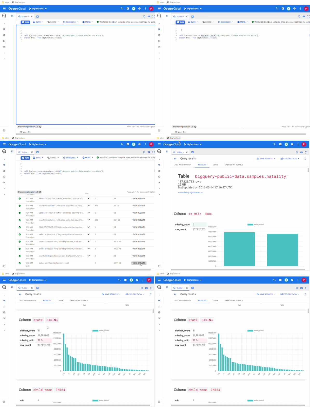
BigQuery, with native and remote routines, is really powerful. But sometimes SQL can be limiting and it cannot work or is too time-consuming for several special cases (e.g. Creating fake datasets, Removing personal data, Array transformations, String transformations, etc.).
This is where BigFunctions comes into play. An open-source package of pre-defined BigQuery-compatible functions. BigFunctions are open-source BigQuery routines that give you SQL superpowers in BigQuery. All BigFunctions represented by a ‘yaml’ file in bigfunctions folder are automatically deployed in public datasets so that you can call them directly without installing them from your BigQuery project. To explore available BigFunctions and to get started, visit the BigFunctions website.
ROLLUP instead of UNION
Using the ROLLUP function you can generate cross-joins avoiding the use of long UNION ALL SQL queries. Imagine having a table like the following:
| Device | OS | Visits |
| Mobile | Android | 5 |
| Mobile | iOS | 10 |
| Tablet | Android | 5 |
| Tablet | iOS | 10 |
| Desktop | Windows | 5 |
| Desktop | macos | 5 |
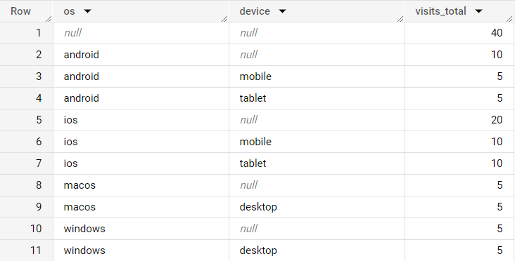
You can use the following SQL query to calculate both the totals by OS and the totals for all OS & device combinations:
SELECT
  os,
  device,
  SUM(visits) AS visits_total
FROM
  datatable
GROUP BY
  ROLLUP(os, device)
ORDER BY
  OS
The result would look like the following table:
Travel back in time

BigQuery allows you to view table data as of a previous point in time, within a pre-defined travel window (by default set to 7 days). Let’s say for instance that you have a table with 10 rows of data on Jan 1st and on Jan 2nd you add 10 more rows of data.
You can use the following SQL query to count the number of rows that were available for that table on Jan 1st:
SELECT Count(*) FROM `condenast-baresquare.qa_automation.output`

FOR SYSTEM_TIME AS OF TIMESTAMP('2023-08-25 00:00:00.000 UTC')
You can also change the travel window on a dataset level using the following SQL query:
ALTER SCHEMA your_table_name
       SET OPTIONS (
              max_time_travel_hours = your_number_of_hours_here
       );
Or you can even join tables using the time travel option just by including the FOR SYSTEM_TIME AS OF clause after the table name in your SQL query.
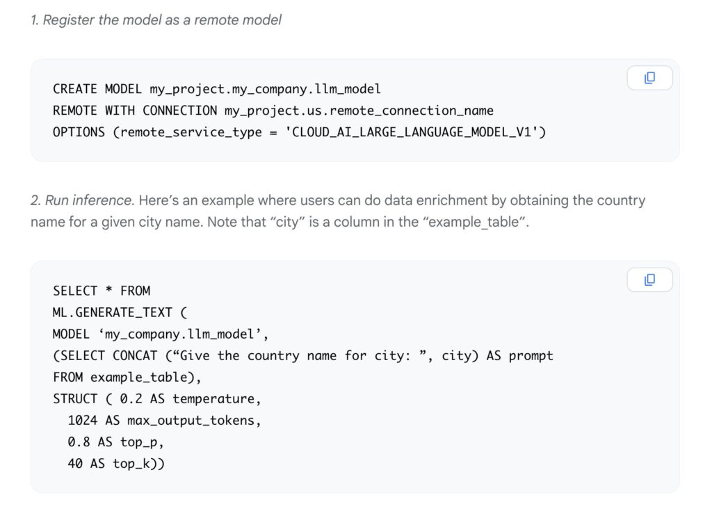
Use LLMs in SQL
The integration of VertexAI Foundation Models in BigQuery makes it easy for businesses to use ML to analyze their data – This can help you to improve your operations, make better decisions, and gain a competitive advantage. For instance, you can do:
- Content generation: Analyze customer feedback and generate personalized email content right inside BigQuery without the need for complex tools
- Summarization: Summarize text stored in BigQuery columns such as online reviews or chat transcripts
- Data enhancement: Obtain a country name for a given city name
- Rephrasing: Correct spelling and grammar in textual content such as voice-to-text transcriptions
- Feature extraction: Extract key information or words from large text files such as in online reviews and call transcripts
- Sentiment analysis: Understand human sentiment about specific subjects in a text
Learn more here
Watch demo here
Step-by-step tutorial here
Codelab tutorial here
Source: https://www.linkedin.com/in/jansmerhovsky/
Analyze job history
Did you know that you can just use an SQL query to collect the complete history of jobs/queries executed against your project? The INFORMATION_SCHEMA.JOBS view contains near real-time metadata about all BigQuery jobs in the current project.
You can use an SQL query like the following to get the list of SQL queries ordered by each user (see sample query below) or even an approximation of the cost for each query by using the total_bytes_billed and total_bytes_processed columns. This would allow you to create a dashboard with statistics, alerts on cost or even report on the most used columns.
SELECT
  user_email,
  query
FROM
  `region-us.INFORMATION_SCHEMA.JOBS`
WHERE
  creation_time >= TIMESTAMP_SUB(CURRENT_TIMESTAMP(), INTERVAL 1 HOUR)
  AND creation_time < TIMESTAMP_ADD(CURRENT_TIMESTAMP(), INTERVAL 1 HOUR)
The underlying data is partitioned by the creation_time column and clustered by project_id and user_email. The query_info column contains additional information about your query jobs. You can find the complete schema here.
QUALIFY: Filtering window function results
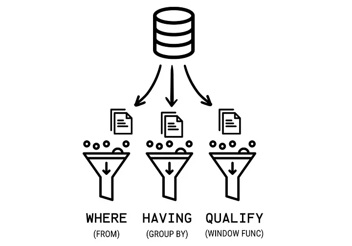
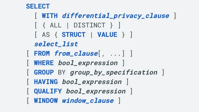
QUALIFY is used to filter your data based on the results of window functions.
In other words, it is to window functions what HAVINGi s to GROUP BY and WHERE is to FROM.
Object Tables: Select files from buckets using SQL
BigQuery object tables are a specialized table type in Google BigQuery that allow you to store and query semi-structured data containing nested and repeated fields, similar to JSON objects, directly within BigQuery’s columnar storage format. They are particularly useful because they enable organizations to work with complex, hierarchical data structures without having to flatten them into traditional relational tables, which can be inefficient and harder to maintain. Object tables bridge the gap between document stores and analytical databases by supporting native querying of nested data using SQL, making it easier to analyze data from sources like IoT devices, web events, or application logs that naturally produce nested structures, while still maintaining BigQuery’s high performance for analytical workloads and ability to handle large-scale data analysis.
You can create an object table using an SQL query:
CREATE EXTERNAL TABLE `my_dataset.object_table`
WITH CONNECTION `us.my-connection`
OPTIONS(
  object_metadata = 'SIMPLE',
  uris = ['gs://mybucket/*'],
  max_staleness = INTERVAL 1 DAY,
  metadata_cache_mode = 'AUTOMATIC'
);
The resulting table will look like the following example:
------------------------------------------------------------------------------------------------------------------------------------------------
|  uri                 | generation | content_type | size  | md5_hash   | updated                        | metadata...name | metadata...value  |
—-----------------------------------------------------------------------------------------------------------------------------------------------
| gs://mybucket/a.jpeg | 165842…    | image/jpeg   | 26797 | 8c33be10f… | 2022-07-21 17:35:40.148000 UTC | null            | null              |
—-----------------------------------------------------------------------------------------------------------------------------------------------
| gs://mybucket/b.bmp  | 305722…    | image/bmp    | 57932 | 44eb90cd1… | 2022-05-14 12:09:38.114000 UTC | null            | null              |
—-----------------------------------------------------------------------------------------------------------------------------------------------
This allows you now to easily work with unstructured data and convert them to structured datasets using BigQuery functionalities. A few sample use cases:
- Use the Document AI API to extract document insights (
ML.PROCESS_DOCUMENTfunction) - Use the Speech-to-Text API to transcribe audio files (
ML.TRANSCRIBEfunction) - Use the Cloud Vision API to annotate images (
ML.ANNOTATE_IMAGEfunction)
More technical details available here.

